Lecture 2.1 notes on Introduction to Computer Vision by Andreas Geiger
- Geometric primitives are the basic building blocks used to describe 3D shapes.
2D points
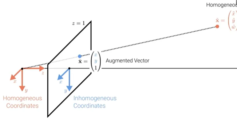
2D points can be written in inhomogeneous coordinates as :
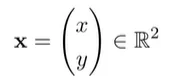
or in homogeneous coordinates as:
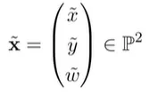
where \(\mathcal{P}^2 = \mathcal{R}^3 \ \{(0, 0, 0)\}\) is called projective space.
Homogeneous vectors that differ only by scale are considered equivalent and define an equivalence class. Homogeneous vectors are defined only up to scale.
An inhomogeneous vector x is converted to a homogeneous vector x as follows:
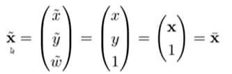
with augmented vector \(\bar{x}\). To convert in the opposite direction we divide by \(\tilde{w}\):
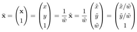
Homogeneous points whose last element is \(\tilde{w} = 0\) are called ideal points or points at infinity. These points can’t be represented with inhomogeneous coordinates.
2D lines can also be expressed using homogeneous coordinates \(\mathcal{I} = (a, b, c)^T\):
\[\{\bar{x} | \tilde{I}^T\bar{x} = 0\} <-> \{x, y | ax + by + c = 0\}\]| We can normalize \(\textbf{\tilde{I}}\) so that \(\tilde{I} = (n_x, n_y, d)^T = (\textbf{n}, d)^T\) with $$ | n | _2 = 1$$. In this case, n is the normal vector perpendicular to the line and d is the distance to the origin. |
An exception is the line at infinity \(\tilde{I_{\inf}} = (0, 0, 1)^T\) which passes through all ideal points.
Cross Product
Cross product expressed as the product of a skew-symmetric matrix and a vector

2D Line Arithmetic
In homogeneous coordinates, the intersection of two lines is given by:
\[\tilde{x} = \tilde{I}_1 x \tilde{I}_2\]